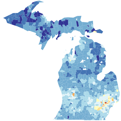
I recently put together an interactive choropleth of Michigan using American Community Survey (ACS) data from the U.S. Census. It looks like this (click on it or here for the actual interactive version):

Here are the steps to create a similar map. Please let me know if there are easier ways:
- **Download shapefiles from the Census.** [You can get any granularity](https://www.census.gov/cgi-bin/geo/shapefiles2010/main) down to ZCTA (the Census' version of ZIP codes), but beware, the larger the area you request, and the more detail, the greater the file size. The ZCTA file of the entire U.S. is more than a gigabyte. (I learned this step from [here](https://github.com/jgoodall/us-maps)).
For this map, I chose ZIP Code Tabulation Areas for the state of Michigan.
- **Get some data for your map.** You can do that in the [American FactFinder](https://www.census.gov/data.html). After finding the data you want, you need to narrow it down to match your geography selection, and then download that .csv file.
For this map, I headed to Advanced Search in FactFinder, searched for Median Rent (B25058), selected a geography of 5-Digit ZIP Code Tabulation Area, narrowed that to those ZCTAs within the state of Michigan, and refined the search. Under the table view of this data, I selected to download it with the data and annotations in a separate file.
- **Join your shapefile and data.**
To do this, you can download free GIS software, QGIS, which allows you to open up a shapefile and attach the data. There are other, more code-based ways of doing this that I tried, but failed to achieve.
For this map, in QGIS, I created a new project, and added a vector layer, selecting the file ending in “zcta510.shp”. This gave me the ZCTA outlines. Then I added in the ACS median rent data by adding another vector layer, and selecting the file “ACS_14_5YR_B25058.csv”. To join the layers, I right clicked on the ZCTA layer and selected properties. On the Joins tab, I clicked the green plus. The ACS data was already selected as the join layer, and for the join field I chose “GEO.id2”. This GEO.id2 matched the ZCTAs in our shapefile. The target field I then chose was “ZCTA5CE10”– which made sure the right areas matched with the right rents. I clicked okay, and the data and map were joined.
Now, still within the properties of the ZCTA layer, I selected style, and selected Categorized from the dropdown at the top. I could then select the data on which to stylize the map – for this, it was “ACS_…HD01_V01”, which corresponded to the column in the ACS .csv of median rent. I choose some nice colors for the color ramp, and hit classify, which automatically filled in categories of rents to shade your map. I hit OK, and the map took on colors by median rent.
- **Export your data for web presentation** While you can see your map with properly shaded ZCTAs by rent in your GIS software, you need to get the map on a webpage. To do this, you need to export your map to a new shapefile, and convert the shapefile to a friendlier format for the web, like geoJSON or the much smaller file format of topoJSON.
For this map, in QGIS, I right-clicked on the ZCTA layer, and saved as an ESRI shapefile. I then ran commands to convert this shapefile to geoJSON using gdal and ogr2ogr, and further converted the geoJSON to the more manageable topoJSON (instructions here).
If you don’t know how to run commands, or have much terminal experience, there are a few web tools available. First, you can take your shapefile and upload to mapshaper.org – make sure to include your .shp, .dbf, .prj, and .shx, or you’ll lose the rent data. Mapshaper will show you the map, without data (don’t worry!), and then you can select export, to geoJSON. Mapshaper says it can export to topoJSON, but I had trouble with using the resulting file (to get the final .json file size down from MB to KB, I had to use the command line conversion tools above).
You can then take this geoJSON to Mapstarter, and play around with how you want the map to look. The choropleth option is available in the colors tab. Mapstarter then allows you to export your map with all the code you need for a pretty web-based, interactive version built on d3.js, which you can further customize.